anuga to landlab: example 2
In this example we use Anuga to create a mesh with variable resolution. With Anuga, we are able to specify regions and specific grid cell resolutions within those regions. In this example we will demonstrate this by doing the following:
Creation of an Anuga mesh with 2 regions of different resolutions
Create simple ridge that is in the center of the domain and each slope has a different cell resolution
Translate the Anuga mesh to a landlab grid
Run the landlab flow accumulation routine
Fill in elevation holes that were created in the mesh generation
Re-run the flow accumulation routine
Import libraries
This notebook requires the numpy, matplotlib, landlab and anuga packages. See the documentation for links to the source installation guides.
import numpy as np
import matplotlib.pyplot as plt
import anuga
import anuga.utilities.idwinterp as idt
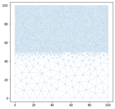
Generate the Anuga mesh
To generate the Anuga mesh we first define a bounding polygon that
defines the outer extents. Then a region within the domain is defined
c_region by listing points in counter-clockwise order that form a
closed shape. The resolution (cell area) is defined for a low resolution
and higher resolution region. Then the mesh is visualized so this
distinction in resolution can be observed.
# define domain extents
bounding_polygon = [[0.0, 0.0],
                    [100.0, 0.0],
                    [100.0, 100.0],
                    [0.0, 100.0]]
# define a region of the domain to model in higher-res
c_region = [[0.0, 50.0], [100.0, 50.0], [100.0, 100.0], [0.0, 100.0]]
# define boundaries
boundary_tags = {'bottom': [0,1],
                'right': [1,2],
                'top': [2,3],
                'left': [3,0]}
# define low and high res values
low_res = 50
high_res = 1
# create the domain
domain = anuga.create_domain_from_regions(bounding_polygon,
                                          boundary_tags,
                                          maximum_triangle_area=low_res,
                                          interior_regions=[[c_region, high_res]],
                                          mesh_filename='test.msh')
# visualize mesh
dplotter = anuga.Domain_plotter(domain)
plt.figure(figsize=(6,6))
plt.triplot(dplotter.triang, linewidth=0.2)
plt.axis('equal')
plt.show()
Figure files for each frame will be stored in _plot
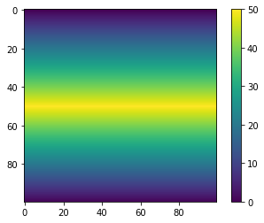
Generate fake topography and assign to the mesh
Here we generate a simple sloped topography. This is defined using numpy, so it is on a regular grid. Built-in interpolation functionality from anuga is applied to interpolate from the regular grid to the anuga mesh. Lastly the elevation values are assigned to the mesh.
# create fake topography as a grid
topo_gridded = np.zeros((100, 100))
[a, b] = np.shape(topo_gridded)
for i in range(0, b):
    if i < b/2:
        topo_gridded[i, :] = i
    else:
        topo_gridded[i, :] = np.abs(i - 100)

grid_y, grid_x = np.mgrid[0:100, 0:100]

plt.figure()
plt.imshow(topo_gridded)
plt.colorbar()
plt.show()
# flatten
xval = grid_x.flatten()
yval = grid_y.flatten()
topoval = topo_gridded.flatten()
# interpolate gridded values to irregular grid
idwtree = idt.invdisttree(np.transpose((xval, yval)), topoval)
topo = idwtree(domain.centroid_coordinates, nnear=3, eps=0, p=1, weights=None)
# set values
domain.set_quantity('elevation', topo, location='centroids')
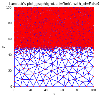
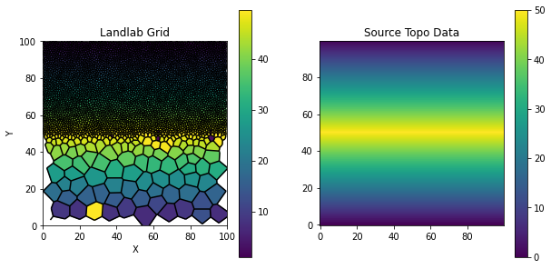
Translate to landlab
To translate the mesh as well as the elevation values from anuga to
landlab, first we need to identify the vertex coordinates and their
corresponding elevation values. After that the
landlab.VoronoiDelaunayGrid object is established using the
coordinate values. This grid is plotted to ensure that the variable
resolution is preserved. Then the elevation attribute is initialized for
each node, and the translation of anuga elevation values to the
landlab grid takes place. The resulting landlab grid with elevations
is plotted next to the source elevation data to visually check them.
# get vertex coordinates and their elevation values
e = domain.get_quantity('elevation')
X, Y, A, V = e.get_vertex_values()
XY = np.column_stack((X,Y))
from landlab.grid import VoronoiDelaunayGrid
from landlab.plot.graph import plot_graph
worked = 0
while worked <= 25:
    try:
        grid = VoronoiDelaunayGrid(X,Y)
        worked = 100
    except Exception:
        worked += 1

print(worked)
100
plt.figure(figsize=(5, 5))
plt.title("Landlab's plot_graph(grid, at='link', with_id=False)")
plot_graph(grid, at="link", with_id=False)
z_vals = grid.add_zeros("topographic__elevation", at="node")
# translating elevation from anuga grid to landlab grid
for i in range(0, len(grid.node_x)):
    ind = np.where(XY==[grid.node_x[i],grid.node_y[i]])[0][0]
    grid.at_node['topographic__elevation'][i] = A[ind]
from landlab.plot.imshow import imshow_grid
plt.figure(figsize=(10,5))
plt.subplot(1,2,1)
plt.title('Landlab Grid')
imshow_grid(grid, 'topographic__elevation', show_elements=True, cmap='viridis')
plt.subplot(1,2,2)
plt.title('Source Topo Data')
plt.imshow(topo_gridded)
plt.gca().invert_yaxis()
plt.colorbar()
plt.show()
/home/jayh/miniconda3/envs/espin/lib/python3.8/site-packages/landlab/plot/imshow.py:267: MatplotlibDeprecationWarning: You are modifying the state of a globally registered colormap. In future versions, you will not be able to modify a registered colormap in-place. To remove this warning, you can make a copy of the colormap first. cmap = copy.copy(mpl.cm.get_cmap("viridis"))
  cmap.set_bad(color=color_for_closed)
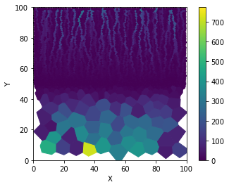
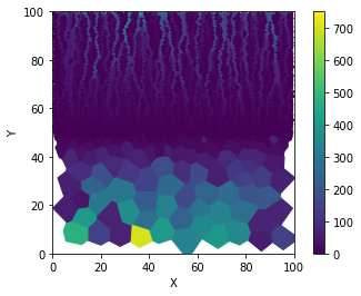
Running the flow accumulator
Now the landlab.FlowAccumulator module is initialized and run. Using
this on the variable resolution grid shows the impact grid resolution
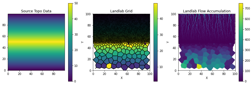
can have on model results (even on a simple sloped topography). The
final cell plots the source elevation data on the left, the generated
landlab grid with elevations in the center, and the resulting flow
accumulation map on the right.
from landlab.components import FlowAccumulator
from landlab.components import FlowDirectorSteepest
fa = FlowAccumulator(grid, 'topographic__elevation',
                     flow_director=FlowDirectorSteepest)
fa.run_one_step()
imshow_grid(grid, 'drainage_area', show_elements=False, cmap='viridis')
from landlab.plot.imshow import imshow_grid
plt.figure(figsize=(15,5))
plt.subplot(1,3,1)
plt.title('Source Topo Data')
plt.imshow(topo_gridded)
plt.gca().invert_yaxis()
plt.colorbar()
plt.subplot(1,3,2)
plt.title('Landlab Grid')
imshow_grid(grid, 'topographic__elevation', show_elements=True, cmap='viridis')
plt.subplot(1,3,3)
plt.title('Landlab Flow Accumulation')
imshow_grid(grid, 'drainage_area', show_elements=False, cmap='viridis')
plt.show()
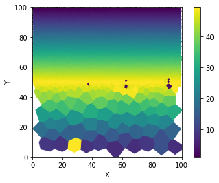
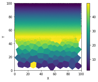
Hole filling
If we look closely at the center panel in the figure above, we might
notice that some cells near the ridge have low elevation values. This is
likely due to the conversion process between the mesh types, leaving
some unintended ‘holes’ in the topography. While this is not ideal, it
is not too different from the ‘holes’ that are commonly found in DEMs.
As such, there are built-in landlab components for dealing with
‘holes’. We will first visualize the domain to see the holes, then apply
the landlab.LakeMapperBarnes component to fill in the holes, and
take a look at the resulting grid.
imshow_grid(grid, "topographic__elevation", show_elements=False, cmap='viridis')
plt.show()
from landlab.components import LakeMapperBarnes
z_init = z_vals.copy()
lmb = LakeMapperBarnes(grid, method='Steepest', surface=z_init, fill_flat=True,
                       redirect_flow_steepest_descent=False, track_lakes=False, ignore_overfill=True)
lmb.run_one_step()
imshow_grid(grid, "topographic__elevation", show_elements=False, cmap='viridis')
plt.show()
Re-running the FlowAccumulator
It is worth noting that the holes predominantly appeared in the ‘coarse’
region of the mesh, and therefore could be due to large irregular cells
whose values were interpolated from a finer regular grid. Anyway, now
that the holes are filled, we can re-run the landlab.FlowAccumulator
component and take a look at how grid resolution impacts our results.
fa = FlowAccumulator(grid, 'topographic__elevation',
                     flow_director=FlowDirectorSteepest)
fa.run_one_step()
imshow_grid(grid, 'drainage_area', show_elements=False, cmap='viridis')